Aggr() in Qlik Sense: the virtual table and its four pitfalls

A virtual table

Aggr(Sum(Sales), Customer) computes Sum(Sales) for each customer and stores the results in an invisible virtual table, one row per customer. A second function, the outer aggregation, then reduces this table to a single value.

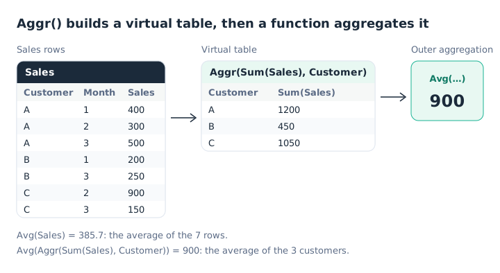
Two averages, two different questions.

Avg(Aggr(Sum(Sales), Customer))   // average sale per customer: 900
Avg(Sales)                        // average sale per row: 385.7

The full syntax:

Aggr({set} [DISTINCT | NODISTINCT] expression, dimension1 [, dimension2 …])

Each dimension must be a field: an expression is not accepted. A dimension can carry a sort order, which we come back to below.

The four pitfalls

In “Pitfalls of the Aggr function” (2015), Henric Cronström lists four. They explain most unexpected results.

1. Forgetting the inner aggregation. The first argument is a measure: it needs an aggregation function. Aggr(Sales, Customer) is treated as Aggr(Only(Sales), Customer), which returns NULL as soon as a customer has several different sales.

2. Forgetting the outer aggregation. Aggr() returns several values. Without a function around it, Qlik applies Only(), and the measure is NULL as soon as there is more than one value, especially on the totals row. Always write Sum(Aggr(…)), Avg(Aggr(…)) or Max(Aggr(…)).

3. Putting set analysis at one level only. Selections apply to both levels, but set analysis only applies where it is written. To calculate on product P1 only, repeat it:

Avg({<Product = {'P1'}>} Aggr({<Product = {'P1'}>} Sum(Sales), Customer))

With the set on the outside only, the virtual table is computed without the filter.

4. Choosing too coarse a grain. The dimensions of Aggr() must be the same as the chart’s, or finer. An Aggr() by month works in a chart by year. The reverse does not: the year’s value shows on one month only, and the others are 0.

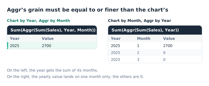
A grain finer than the chart works; a coarser one does not.

To show the customer’s total on every row of a customer × product table, there are two options: Sum(TOTAL <Customer> Sales), the simplest, or Aggr(NODISTINCT Sum(Sales), Customer). The NODISTINCT qualifier returns the value on every row of the combination, instead of only one.

What Aggr makes possible

Counting and filtering on an intermediate result. Customers above €1,000:

Sum(Aggr(If(Sum(Sales) > 1000, 1, 0), Customer))

An expression search in set analysis gives the same result, often faster: Count({<Customer = {"=Sum(Sales) > 1000"}>} DISTINCT Customer). It is covered in our article on advanced set analysis.

Creating a calculated dimension. A dimension that only shows the two best customers:

=Aggr(If(Rank(Sum(Sales)) <= 2, Customer), Customer)

Untick Include null values to hide the others.

Accumulating in a controlled order. An Aggr() dimension can carry a sort. This is what makes a running total computed with inter-record functions reliable, whatever the chart’s sort order:

Sum(Aggr(RangeSum(Above(Sum(Sales), 0, 12)), (Month, (NUMERIC, ASCENDING))))

The sort types are NUMERIC, TEXT, FREQUENCY and LOAD_ORDER, with ASCENDING or DESCENDING. The Qlik help notes that, without a sort, the same expression does not accumulate correctly.

The cost

Each evaluation of Aggr() builds its virtual table. On a large table, with several dimensions, this is expensive, and the calculation is redone on every selection. If the intermediate result does not depend on selections, such as a customer’s all-time total, compute it in the script instead.

Key takeaways

• Two levels of calculation. Aggr builds a virtual table, an outer aggregation reduces it.
• One aggregation inside, one outside. Otherwise Qlik applies Only() and returns NULL.
• Set analysis at both levels. A filter written outside does not filter the virtual table.
• An equal or finer grain. Aggr’s dimensions must be the chart’s, or more detailed.
• A sort for running totals. (Month, (NUMERIC, ASCENDING)) fixes the virtual table’s order.
• The script when possible. A result that does not depend on selections is computed at load time.

Try it in Qlik Sense

This script replays the article’s examples with the data from the diagrams, loaded INLINE: it needs no file and no database. Paste it into the data load editor of an empty app and reload. The expressions to try are in comments: build the charts described on a sheet.

// Aggr() in Qlik Sense: try-it script (HeyData)
// Paste it into the data load editor of an empty app, reload,
// then build the charts described below on a sheet.
Sales:
LOAD * INLINE [
Year, Month, Customer, Product, Sales
2025, 1, A, P1, 400
2025, 2, A, P2, 300
2025, 3, A, P1, 500
2025, 1, B, P1, 200
2025, 3, B, P2, 250
2025, 2, C, P2, 900
2025, 3, C, P1, 150
];

// KPIs:
//   Avg(Aggr(Sum(Sales), Customer))                              → 900 (first diagram)
//   Avg(Sales)                                                   → 385.7
//   Sum(Aggr(If(Sum(Sales) > 1000, 1, 0), Customer))             → 2 (A and C)
//   Max(Aggr(Sum(Sales), Customer))                              → 1200
//   Avg({<Product = {'P1'}>} Aggr({<Product = {'P1'}>} Sum(Sales), Customer))   → 416.7
//
// Table by Month (second diagram, right):
//   Sum(Aggr(Sum(Sales), Year))     → 2700 on a single month, 0 elsewhere
//   Sum(Aggr(Sum(Sales), Year, Month))  → 600, 1200, 900
//
// Table by Month, sorted running total:
//   Sum(Aggr(RangeSum(Above(Sum(Sales), 0, 12)), (Month, (NUMERIC, ASCENDING))))   → 600, 1800, 2700
//
// Table by Customer and Product:
//   Aggr(NODISTINCT Sum(Sales), Customer)   → the customer total on every row
//
// Calculated dimension (the two best customers):
//   =Aggr(If(Rank(Sum(Sales)) <= 2, Customer), Customer)   → A and C

Sources

• Qlik Cloud help: Aggr - chart function, syntax, NODISTINCT and dimension sorting.
• Henric Cronström, Qlik Design Blog: Pitfalls of the Aggr function, October 2015.

Text and examples are by HeyData. This article is part of our series on lesser-known Qlik Sense functions and keywords: explore the series.