
· By HeyData team
Series: Henric Cronström’s Technical Briefs, revisited for Qlik Sense · article 1 of 7
Joins and lookups in Qlik Sense: when to link, when to join
In Qlik Sense, two tables can be linked in two ways: through an association in the data model, or through a join in the script. The choice looks technical. Yet it decides how much memory is used, how readable the script is and, above all, whether Sum() and Count() return the right numbers.
This article summarises the Technical Brief “Joins and Lookups” by Henric Cronström (Qlik, September 2012) and adapts it to Qlik Sense. His technical papers remain references: we revisit them with today’s tools.
The problem
Most query tools produce a single denormalised table: a SELECT can read several tables, but it returns only one. The Qlik engine works differently. It keeps several tables in memory and links them through the names of the key fields.
Developers coming from SQL therefore have a reflex: join everything in the script. Sometimes that is justified. Often it leads to duplicated rows and wrong totals. You need to tell three tools apart: the association, the join and the lookup function.
Association or join: the difference
An association is a link between two tables that share a field with the same name. It is not a join yet: it is only evaluated when the user makes a selection. A join (the Join prefix) runs during the reload. Its result is a single table in the data model.
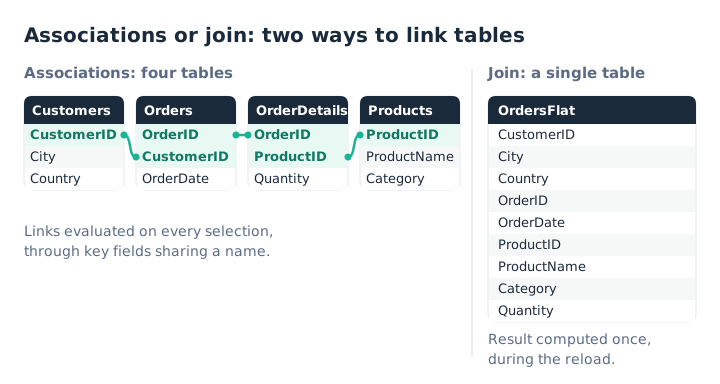
Associations evaluated on selection, or one table computed at reload.
Three differences follow:
- Timing: the association is computed on demand, the join once and for all at reload.
- Nature: a join is explicitly inner, outer, left or right. An association changes with the context. With no selection, it behaves like a full outer join. If you select some customers, it acts as a left join: all selected customers remain possible, even without orders, but only their orders are possible.
- Condition: an association is always a natural join, based on equal values. A condition such as
TableA.Key >= TableB.Keyis impossible.
In Qlik Sense, the data model viewer shows these associations. The Data Manager also offers them visually. The developer’s job stays the same: give keys identical names so they link, and give every other field a unique name to avoid unwanted links.
Joins in the script
The danger: the row count changes
Joining two tables can change the number of rows. That is often intended. Joining order headers to their lines (a one-to-many relationship) gives as many rows as the detail table. The price: an amount held by the header, such as freight, can no longer be summed directly. With a many-to-many relationship, the result may be larger than either source table.
The real trap is a relationship you believe is one-to-one when it is actually one-to-many. Product attributes stored in a separate table are the typical case: one product can have several attributes.
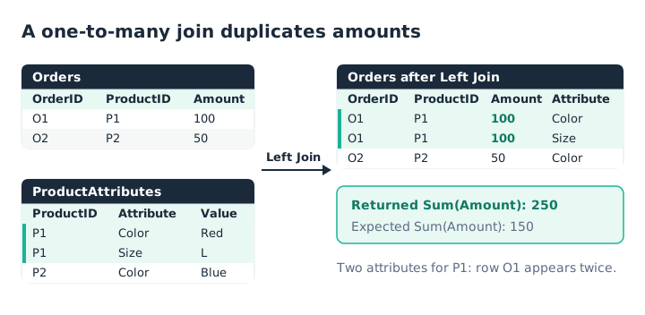
One product with two attributes, and order O1 counts twice.
The engine is not wrong: it sums exactly what is in the table. It is the model that no longer says what you think.
The SQL join, run by the database
A join written inside an SQL SELECT is sent as is to the connector. Qlik Sense does not interpret the query: the database runs it. The syntax therefore depends on the DBMS. This option is often more efficient on large volumes. It also accepts non-natural joins, with inequalities.
LIB CONNECT TO 'Sales_DB';

SalesPerCustomer:
SQL SELECT c.CustomerID, c.CustomerName, SUM(s.SaleAmount) AS SalesAmount
FROM Customers c
LEFT JOIN Sales s ON c.CustomerID = s.CustomerID
GROUP BY c.CustomerID, c.CustomerName;
The Join prefix, run by Qlik
The Join prefix combines the table being loaded with a table already loaded. The join is natural: it uses the fields that share a name. With no common field, you get the Cartesian product of both tables. By default the join is outer. Inner, Left and Right change its type.
Orders:
LOAD OrderID, CustomerID, OrderDate
FROM [lib://Data/Orders.qvd] (qvd);

Left Join (Orders)
LOAD CustomerID, CustomerName, Country
FROM [lib://Data/Customers.qvd] (qvd);
This join is fast but memory-hungry. It suits small tables well. On large tables, a join in the database is often preferable.
The Keep prefix, to filter without merging
Keep compares the tables like a join but leaves them separate. It only removes the rows a join would have discarded. It must be preceded by Inner, Left or Right. A classic case: you load only part of the transactions, then only the matching products.
OrderDetails:
LOAD * FROM [lib://Data/OrderDetails.qvd] (qvd)
WHERE OrderDate >= MakeDate(2026, 1, 1);

Products:
Left Keep (OrderDetails)
LOAD * FROM [lib://Data/Products.qvd] (qvd);
Lookup functions
Many joins are really used to translate a value: getting the category from the product ID. Only one value is expected per key. For this need, the author is clear: avoid the join and use a lookup function. The script runs faster and the row count does not move. If several values are expected per key, a lookup function is the wrong tool: it only returns the first one found.
ApplyMap(), the default choice
ApplyMap() relies on a two-column mapping table: the source value, then the target value. Column names do not matter. The mapping table is dropped automatically at the end of the script. The third parameter, which is recommended, sets the value returned when the key is missing.
Map_Category:
Mapping LOAD ProductID, Category
FROM [lib://Data/Products.qvd] (qvd);

OrderData:
LOAD *,
    ApplyMap('Map_Category', ProductID, 'Missing') AS Category
FROM [lib://Data/OrderData.qvd] (qvd);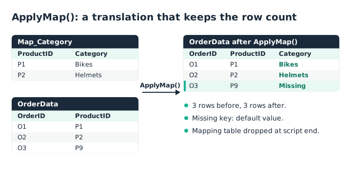
ApplyMap() adds a field without adding a row.
Its only drawback: you must prepare the mapping table before using it.
Lookup(), more flexible but slower
Lookup() reads a field from any table already loaded. Field and table names are passed in single quotes. The value searched for, taken from the current table, is not.
OrderData:
LOAD *,
    Lookup('Category', 'ProductID', ProductID, 'Products') AS Category
FROM [lib://Data/OrderData.qvd] (qvd);
It is flexible, but much slower than ApplyMap().
Exists() and Peek(), two special cases
Exists() does not return a value. It tells you whether a value has already been loaded into a field. It is used to exclude rows, or to reduce a master table to the keys already present, like Keep.
Discontinued:
LOAD ProductID AS DiscontinuedID
FROM [lib://Data/DiscontinuedProducts.qvd] (qvd);

Products:
LOAD * FROM [lib://Data/Products.qvd] (qvd)
WHERE NOT Exists(DiscontinuedID, ProductID);
Peek() reads a value by row number: Peek('Category', -1, 'Products') returns the last one. Since you rarely know the useful row number, its use as a lookup remains limited.
Normalise or denormalise?
The author favours a model that is as normalised as possible. His arguments:
- it uses the least memory;
- calculations are generally as fast, sometimes faster;
- a script with few transformations is easier to read and maintain;
- the row count does not change, so
Sum()andCount()stay correct.
That last point matters even more in Qlik Sense, where users build their own visualizations. They should not need to know the subtleties of the model.
The case is not settled, though. An expression such as Sum(Price * Quantity), whose fields sit in two tables, forces the engine to build a join in memory at calculation time. If those tables are far apart in the model, joining in the script can improve response times. With modest dimension tables, the gap is usually marginal. Two large linked tables, such as order headers and order lines, often benefit from being joined. Header fields can then only be counted with Count(DISTINCT …), which is slower on a large table.
The author’s conclusion fits in one sentence: “The best join is often the one that never is made” (Henric Cronström). Often, but not always.
Key takeaways
- Associate by default. The model links tables through key names. Only join for a clear reason.
- Check the cardinality. A relationship assumed to be one-to-one that is actually one-to-many duplicates rows and skews totals.
- ApplyMap() to translate. One value per key, one added field, no extra rows, and a third parameter for missing keys.
- Keep or Exists() to filter. They reduce a table without merging it into another.
- Join for performance, knowingly. Measure the gain, then ask whether the script stays readable and the formulas easy to write.
Try it in Qlik Sense
This script replays the article’s examples with the data from the diagrams, loaded INLINE: it needs no file and no database. Paste it into the data load editor of an empty app, pick an example with the vExample variable, then reload.
// Joins and lookups in Qlik Sense: try-it script
// Based on “Joins and Lookups”, a Technical Brief by Henric Cronström (Qlik, 2012), adapted by HeyData.
// Paste it into the data load editor of an empty app, pick an example,
// reload, then open the data model viewer.
SET vExample = 1;   // 1 to 7

IF $(vExample) <= 2 THEN
    // Examples 1 and 2: four tables linked by CustomerID, OrderID and ProductID (first diagram)
    Customers:
    LOAD * INLINE [
    CustomerID, City, Country
    C1, Lyon, France
    C2, Berlin, Germany
    C3, Madrid, Spain
    ];

    Orders:
    LOAD * INLINE [
    OrderID, CustomerID, OrderDate
    1001, C1, 2026-01-05
    1002, C2, 2026-01-12
    1003, C1, 2026-02-03
    ];

    OrderDetails:
    LOAD * INLINE [
    OrderID, ProductID, Quantity
    1001, P1, 1
    1001, P2, 2
    1002, P2, 1
    1003, P1, 3
    ];

    Products:
    LOAD * INLINE [
    ProductID, ProductName, Category
    P1, Road bike, Bikes
    P2, Helmet, Helmets
    P3, Bell, Accessories
    ];

    IF $(vExample) = 2 THEN
        // Example 2: the same tables joined into one, OrdersFlat
        OrdersFlat:
        NoConcatenate
        LOAD * RESIDENT Customers;
        Left Join (OrdersFlat) LOAD * RESIDENT Orders;
        Left Join (OrdersFlat) LOAD * RESIDENT OrderDetails;
        Left Join (OrdersFlat) LOAD * RESIDENT Products;
        DROP TABLES Customers, Orders, OrderDetails, Products;
        // C3, with no order, keeps one row; P3, never ordered, disappears.
    END IF
END IF

IF $(vExample) = 3 THEN
    // Example 3: a one-to-many join duplicates amounts (second diagram)
    Orders:
    LOAD * INLINE [
    OrderID, ProductID, Amount
    O1, P1, 100
    O2, P2, 50
    ];

    Left Join (Orders)
    LOAD * INLINE [
    ProductID, Attribute, Value
    P1, Color, Red
    P1, Size, L
    P2, Color, Blue
    ];
    // 3 rows: Sum(Amount) returns 250 instead of 150.
END IF

IF $(vExample) = 4 THEN
    // Example 4: Left Keep reduces Products to products ordered since 2026
    OrderDetails:
    LOAD OrderID, ProductID, Date(Date#(OrderDate, 'YYYY-MM-DD')) AS OrderDate
    INLINE [
    OrderID, ProductID, OrderDate
    1000, P3, 2025-12-20
    1001, P1, 2026-01-05
    1002, P2, 2026-01-12
    ]
    WHERE Date#(OrderDate, 'YYYY-MM-DD') >= MakeDate(2026, 1, 1);

    Products:
    Left Keep (OrderDetails)
    LOAD * INLINE [
    ProductID, ProductName
    P1, Road bike
    P2, Helmet
    P3, Bell
    ];
    // Two separate tables; Products now holds only P1 and P2.
END IF

IF $(vExample) = 5 THEN
    // Example 5: ApplyMap translates without adding rows (third diagram)
    Map_Category:
    Mapping LOAD * INLINE [
    ProductID, Category
    P1, Bikes
    P2, Helmets
    ];

    OrderData:
    LOAD *,
        ApplyMap('Map_Category', ProductID, 'Missing') AS Category
    INLINE [
    OrderID, ProductID
    O1, P1
    O2, P2
    O3, P9
    ];
    // 3 rows before, 3 rows after; O3 gets 'Missing'.
END IF

IF $(vExample) = 6 THEN
    // Example 6: Lookup reads a table already loaded
    Products:
    LOAD * INLINE [
    ProductID, Category
    P1, Bikes
    P2, Helmets
    ];

    OrderData:
    LOAD *,
        Lookup('Category', 'ProductID', ProductID, 'Products') AS OrderCategory
    INLINE [
    OrderID, ProductID
    O1, P1
    O2, P2
    O3, P9
    ];
    // O3 has no match: OrderCategory is NULL.
END IF

IF $(vExample) = 7 THEN
    // Example 7: Exists filters out discontinued products
    Discontinued:
    LOAD * INLINE [
    DiscontinuedID
    P3
    ];

    Products:
    LOAD * INLINE [
    ProductID, ProductName
    P1, Road bike
    P2, Helmet
    P3, Bell
    ]
    WHERE NOT Exists(DiscontinuedID, ProductID);

    DROP TABLE Discontinued;
    // Products holds only P1 and P2.
END IF
Source
“Joins and Lookups”, QlikView Technical Brief, Henric Cronström (“hic” on Qlik Community), September 2012, published on Qlik Community in the QlikView Documents section. All credit for the original content goes to him; the adaptation to Qlik Sense and any errors are HeyData’s. This article is part of our review of the Technical Briefs: discover the series.